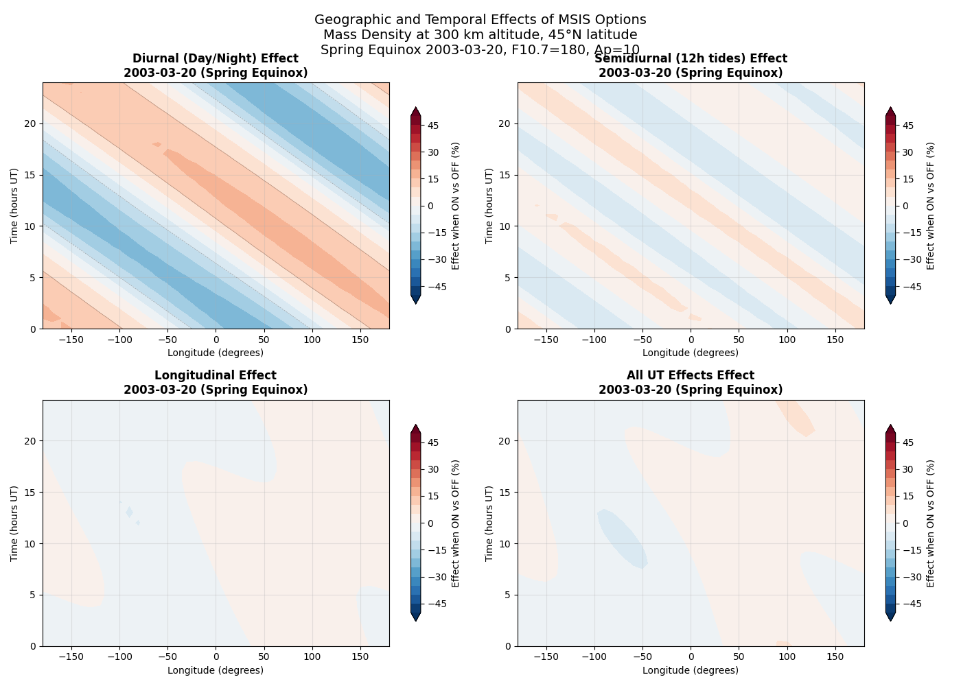
Geographic and Temporal Patterns

This example demonstrates how different MSIS options affect atmospheric density across longitude and time. The plots show surface maps of mass density at 300 km altitude, revealing the geographic and temporal patterns controlled by each option.

Four key MSIS options with strong spatial/temporal patterns are highlighted: 1. Diurnal variations (day/night differences) 2. Semidiurnal tidal effects (12-hour cycles) 3. Longitudinal variations (geographic differences) 4. Universal Time effects (UT dependencies)

This complements the altitude overview by showing horizontal structure patterns.

import matplotlib.pyplot as plt
import numpy as np

import pymsis


# Define grid parameters
lons = np.linspace(-180, 180, 37)  # 10-degree longitude spacing
times = np.linspace(0, 24, 25)  # Hourly through one day
lat = 45  # Mid-latitude
alt = 300  # Thermosphere where effects are clear
f107 = 180
f107a = 160
ap = 10

# Create date array for one day
base_date = np.datetime64("2003-03-20")  # Spring equinox - sun centered on equator
dates = [base_date + np.timedelta64(int(h), "h") for h in times]

# Select key options that show strong geographic/temporal patterns
key_options = {
    "Diurnal (Day/Night)": 6,  # Index 6 = diurnal
    "Semidiurnal (12h tides)": 7,  # Index 7 = semidiurnal
    "Longitudinal": 10,  # Index 10 = longitudinal
    "All UT Effects": 9,  # Index 9 = all UT effects
}

# Create figure with subplots
fig, axes = plt.subplots(2, 2, figsize=(14, 10))
axes = axes.flatten()

# Create aps array for single calculations
aps_single = [[ap] * 7]  # Array of arrays for single date calculations

for plot_idx, (option_name, option_idx) in enumerate(key_options.items()):
    ax = axes[plot_idx]

    # Create meshgrid for plotting
    LON, TIME = np.meshgrid(lons, times)
    density_on = np.zeros_like(LON)
    density_off = np.zeros_like(LON)

    # Calculate density for each lon/time combination
    for i, _ in enumerate(times):
        date = dates[i]

        # All options ON
        options_on = [1] * 25
        result_on = pymsis.calculate(
            date, lons, lat, alt, f107, f107a, aps_single, options=options_on
        )
        density_on[i, :] = np.squeeze(result_on)[:, pymsis.Variable.MASS_DENSITY]

        # Target option OFF
        options_off = [1] * 25
        options_off[option_idx] = 0
        result_off = pymsis.calculate(
            date, lons, lat, alt, f107, f107a, aps_single, options=options_off
        )
        density_off[i, :] = np.squeeze(result_off)[:, pymsis.Variable.MASS_DENSITY]

    # Calculate relative difference (%)
    relative_diff = 100 * (density_on - density_off) / density_on

    # Create contour plot
    levels = np.linspace(-50, 50, 21)
    contour = ax.contourf(
        LON, TIME, relative_diff, levels=levels, cmap="RdBu_r", extend="both"
    )

    # Add contour lines for clarity
    ax.contour(
        LON,
        TIME,
        relative_diff,
        levels=levels[::4],
        colors="black",
        alpha=0.3,
        linewidths=0.5,
    )

    ax.set_title(
        f"{option_name} Effect\n{base_date} (Spring Equinox)",
        fontsize=12,
        fontweight="bold",
    )
    ax.set_xlabel("Longitude (degrees)")
    ax.set_ylabel("Time (hours UT)")
    ax.grid(True, alpha=0.3)

    # Add colorbar
    cbar = plt.colorbar(contour, ax=ax, shrink=0.8)
    cbar.set_label("Effect when ON vs OFF (%)", fontsize=10)

# Add overall title
fig.suptitle(
    f"Geographic and Temporal Effects of MSIS Options\n"
    f"Mass Density at {alt} km altitude, {lat}°N latitude\n"
    f"Spring Equinox 2003-03-20, F10.7={f107}, Ap={ap}",
    fontsize=14,
    y=0.98,
)

plt.tight_layout()
plt.subplots_adjust(top=0.88)
plt.show()