Altitude profiles

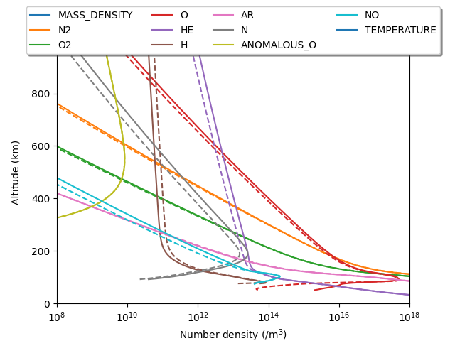
This example demonstrates how to calculate the altitude variations at a single location. Additionally, we show the difference between densities at noon (solid) and midnight (dashed).

import matplotlib.pyplot as plt
import numpy as np

import pymsis


lon = 0
lat = 70
alts = np.linspace(0, 1000, 1000)
f107 = 150
f107a = 150
ap = 7
aps = [[ap] * 7]

date = np.datetime64("2003-01-01T00:00")
output_midnight = pymsis.calculate(date, lon, lat, alts, f107, f107a, aps)
date = np.datetime64("2003-01-01T12:00")
output_noon = pymsis.calculate(date, lon, lat, alts, f107, f107a, aps)

#  output is now of the shape (1, 1, 1, 1000, 11)
# Get rid of the single dimensions
output_midnight = np.squeeze(output_midnight)
output_noon = np.squeeze(output_noon)

_, ax = plt.subplots()
for variable in pymsis.Variable:
    if variable.name in ("Total mass density", "Temperature"):
        # Ignore non-number densities
        continue
    (line,) = ax.plot(output_midnight[:, variable], alts, linestyle="--")
    ax.plot(output_noon[:, variable], alts, c=line.get_color(), label=variable.name)

ax.legend(
    loc="upper center", bbox_to_anchor=(0.5, 1.15), fancybox=True, shadow=True, ncol=4
)
ax.set_title(f"Longitude: {lon}, Latitude: {lat}")
ax.set_xscale("log")
ax.set_xlim(1e8, 1e18)
ax.set_ylim(0, 1000)
ax.set_xlabel("Number density (/m$^3$)")
ax.set_ylabel("Altitude (km)")

plt.show()